What tacos taught me about process optimization

On a recent work trip, I found myself in a taco restaurant near Madison Square Garden. While I was immediately taken with the fact that they had Coca-Cola from Mexico (cane sugar FTW!), I couldn't help but notice that the whole setup—the position of the register, how the line was configured, the table style—was a tangible representation of something I find fascinating: queueing theory.

When you enter the restaurant, you wait in line (far right in the photo) and order from a (single) cashier. Your order is then delivered to one of several folks who make the tacos (counter at the back in the center). From there, you take your order to a set of (standing!) tables to eat (foreground). Then, it being New York, you get the hell out and make space for the next folks.

This layout was particular enough that it got me thinking:

• Why are these tacos so delicious?
• Why is there only one cashier?
• Is three the correct number of taco assemblers?
• Standing tables? WTF?

The delectable taco seasoning may have been a secret family recipe, but the answers to my other questions could probably be traced back to organic developments over several years based on experimentation and lessons learned during peak hours. But I wondered if we could find some more rigorous explanations with queueing theory.

I have what can charitably be described as an unhealthy relationship to needing to know things, so I’m writing a multi-part series on the whys and wherefores of this system, and what we can learn about it when we apply some math. 

The schematic—and our first equation

One of the things I love about queueing theory is that it gives us a language to abstract the specifics of the taco place, or any system where work arrives, is processed, and then leaves. Using these tools we can understand the dynamics that are fundamental to a system, such as standing in line at the airport, or waiting in traffic, or any of a hundred other scenarios.

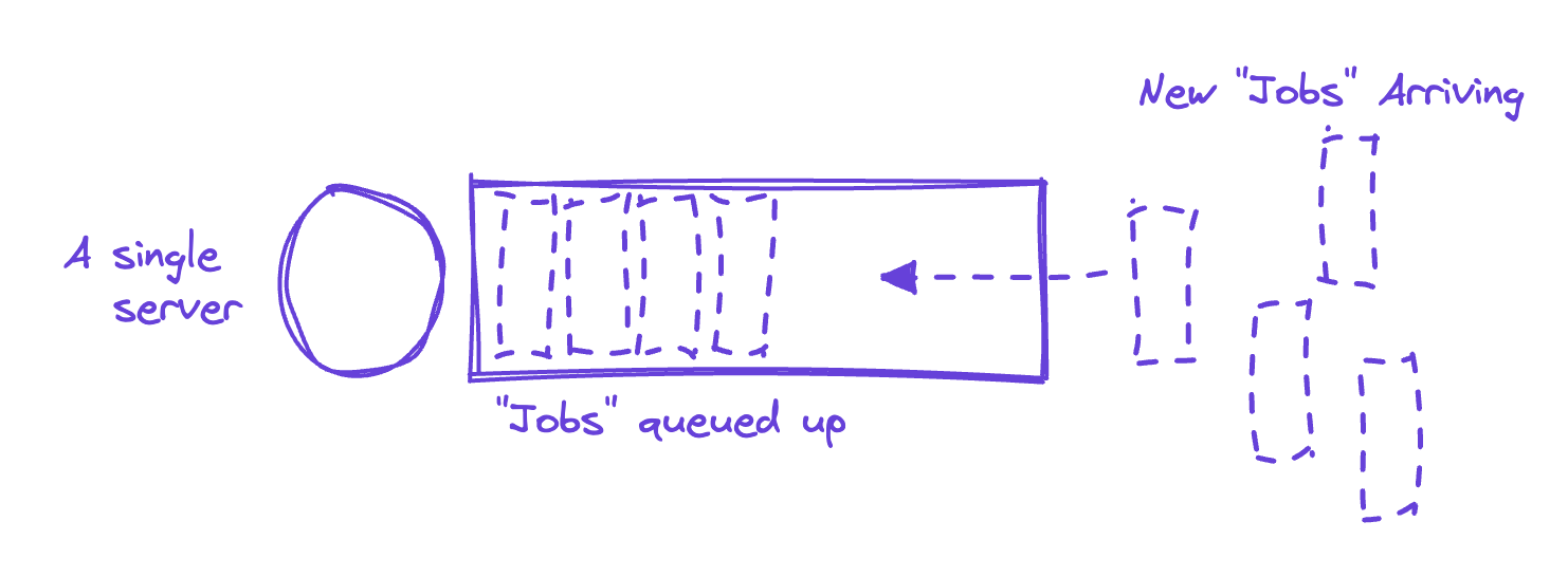
In the case of the restaurant,  we can zoom-out and re-envision it as a giant queue. There are three quantities that describe this system:

• How many people are in the system—this is how crowded the restaurant is, including people waiting, eating, and picking up their food
• How often new customers show up—this is the arrival rate
• How long a customer stays in the store—this is a combination of time spent ordering, prepping, and eating tacos

In 1954 a man named Phillip Morse published the mathematical relationship between these quantities, which is called “Little’s law”:

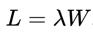
What this equation basically says is that the number of customers in the system (L) is equal to the arrival rate (lambda) multiplied by the average time a customer spends in the system (W). 

And with this formula, we can answer some mission-critical questions.

How big should the restaurant be?

If we were building the restaurant from scratch, we could use this equation to figure out how big to make it. For example, if we know that people take 10 minutes to order and eat, and we’re expecting two to three new people to show up every minute during peak times, then we can estimate how much space we need:

L = 10 * (2 or 3) = 20 or 30 people

In our restaurant, if we had room for fewer than 20 to 30 people, the line would back up and out the door.

Will I make my train?

If we’re hungry and pressed for time and we know how many people are in the restaurant (L) and roughly how long they take (lambda), then we can estimate how long we’re going to wait:

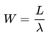
So if we arrive at the taco place and there are two people in line, and it takes 20 minutes to order food, eat, and leave, and only one person can fit in the restaurant at a time, we’re going to be waiting for 2 / (1/20)  = 40 minutes. We might not make our train. 

In reality, it’s a bit more complicated than that…

In practice, the situation is more complex. The restaurant is more accurately modeled as a set of smaller queueing systems, which are each described by their own Little's laws:

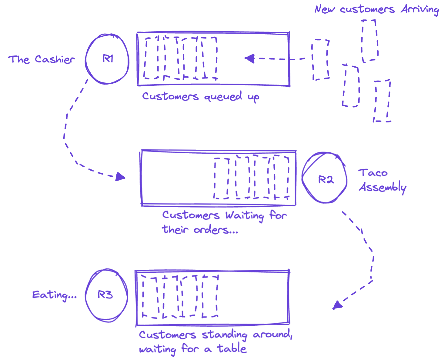
The diagram shows people arriving at the taco place and waiting in line to order. The cashier can handle people at the rate R1. From there, the customers are sent to the taco assembly station, which processes orders at rate R2. From there, customers go to a table and eat, which takes time (R3), and then they leave.

In between each of the processing steps, people are milling around—they’re in line at the door, or they’re waiting for their order, or they’re wandering the seating section with a lost look in their eyes. This is called "buffering" in the biz, which is a fancy way of saying that you have people / work / jobs waiting around to be worked on.

Assuming, as we do in the model, that there is only one cashier, and only one taco assembler, we quickly run into problems. For example, if the person at the register is always faster than the taco assembler, people will start queueing up, filling up the space between the register and the assembly station, eventually resulting in a buffer overflow. In general, we're going to end up needing to solve for the slowest component in the system (hat tip to The Goal).

Theory of Constraints — no savoring allowed

When optimizing the flow, we want to focus on the slowest component. In the case of our taco place, this is the people eating. If you’re trying to speed up a process (any process), there are several knobs you can turn but it usually boils down to two things: do each job faster, or do more jobs at the same time. In the case of speeding up the eating phase, our taco entrepreneurs did both:

• They did more jobs at the same time. There is more than one table, so multiple people are eating at any one point. In our schematic, we would represent this as having more “servers” in the eating stage.
• They did each job faster. They have standing tables so people are less likely to linger. This reduces the service time, which cuts down on the queue.

Work smarter, not harder

The second thing they’d optimized was the taco assembly itself. In this case, they followed the same pattern as the eating phase:

• They did more jobs at the same time.They have more than one assembly station, so there are multiple orders being put together at the same time.
• They made each job faster. They designed a limited menu so each taco can be assembled in a short time.

The more you know, the more you can optimize

Now we can see that the layout of the taco place reflects queueing theory at work. And we can even understand the long-term behavior of the system and start thinking about modifications, like adding more cashiers or advertising a lunchtime deal to bring in more customers, and what the impacts might be.

Keep in mind that Little's law talks about the long-term averages of each quantity. It doesn't take into account the behavior of the system if any of these rates change with time. We fudged this above by assuming the peak-time arrival rate, and average rates everywhere else. In the real world, we know that customers show up in bursts, so the arrival rate changes over time, and that taco assemblers and order takers get tired, so service time changes too.

For the mathematically minded among you, we’ll take a look at some of these dynamics in a later blog.

Until then, you can make your real-life wait times more fun. Next time you’re in a restaurant, or waiting for your car to be serviced, or stuck in traffic, dust off your Little’s law, take a look at the variables at play, and figure out how you could optimize the system.